
In this article, we will learn to create maps in Python using OSM (OpenStreetMap) shapefiles, GeoPandas library, and Matplotlib. I will be using Google Colab notebook for this task.
How to download OSM shapefiles for a region?
We will download the OpenStreetMap (OSM) shapefiles from Geofabrik’s free download server. This server has OpenStreetMap data extracts in various file formats including shapefile. These data extracts are updated almost every day.
Let’s say you want to download a shapefile for Japan, visit https://download.geofabrik.de and select Asia from the list of Sub Regions.
A new page will open up that will have a list of Asian countries. From this list select Japan. You will be taken to another page showing you a list of sub-regions in Japan. Select any region of your choice. I will go ahead with the Chūbu region.
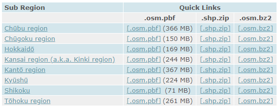
Right-click the .shp.zip link of the Chūbu region and copy the link’s address. Then go to your Colab notebook or terminal and download the zipped shapefile using the following command.
!wget https://download.geofabrik.de/asia/japan/chubu-latest-free.shp.zip
To unzip and extract the shapefiles, you may use the below command. It will extract various shapefiles in your working directory.
!unzip chubu-latest-free.shp.zip
Loading a shapefile using GeoPandas
As discussed earlier, I have downloaded Japan’s spatial data. Now I will use the data of a city in Japan instead of the entire Japan region because it will need less computation resources. So, I will select the city of Nagoya.
import geopandas as gpd
import matplotlib.pyplot as plt

# min-max lat-long coordinates of Nagoya city
longitude_min = 136.793863
latitude_min = 35.036317
longitude_max = 137.039585
latitude_max = 35.243637

bbox = (longitude_min, latitude_min, longitude_max, latitude_max)
As you can see above, I have found the maximum and minimum latitude-longitude values for Nagoya. You can find such coordinates for any city with the help of Google Maps or Google Earth.
Let’s load our first shapefile using GeoPandas.
# load roads shapefile
roads = gpd.read_file("gis_osm_roads_free_1.shp", bbox = bbox)

roads.head()
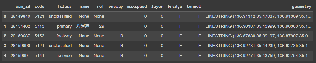
As you can see, we have loaded the shapefile containing the roads shapefile data. The GeoPandas dataframe contains multiple columns, but the important columns are ‘fclass’ and ‘geometry’.
‘fclass’ tells us about the type of road, whether it is a primary road, footway, stairs, or service road. The ‘geometry’ column contains the spatial features that will be used for creating geospatial visualization.
Create a simple map with shapefile data
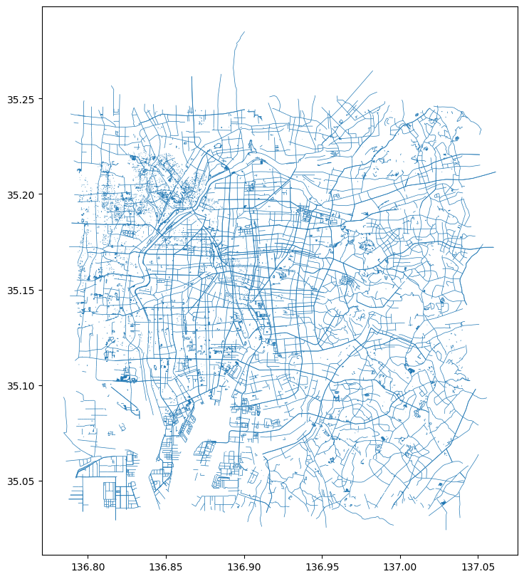
Now we will use the roads spatial data and plot our first map. However, instead of plotting all types of roads, I will use only “primary”, “secondary”, “tertiary”, and “service” roads otherwise it will look messed up.
# Change the size of the plot
fig, ax = plt.subplots(figsize=(10, 10))

# Plot roads
roads[roads['fclass'].isin(["primary", "secondary", "tertiary", "service"])].plot(ax=ax, linewidth=0.5)
Loading different types of shapefiles
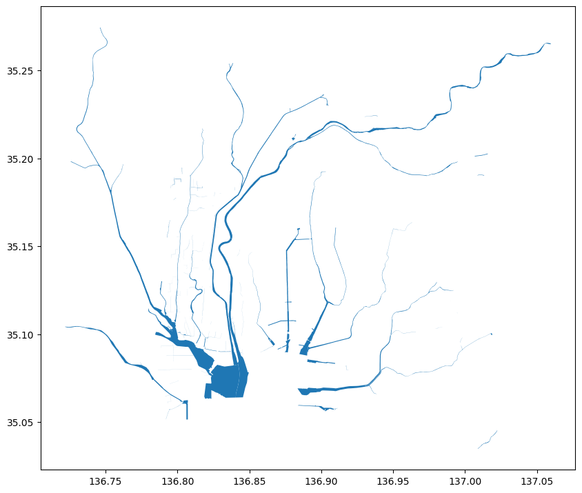
Let’s load other shapefiles as well. The water shapefile seems interesting.
# load water shapefile
water = gpd.read_file("gis_osm_water_a_free_1.shp", bbox = bbox)

water['fclass'].value_counts()

This shapefile consists of different types of water bodies. Let’s use the ‘riverbank’ for visualization.
# Change the size of the plot
fig, ax = plt.subplots(figsize=(10, 10))

# Plot riverbank
water[water['fclass'] == "riverbank"].plot(ax=ax)
Awesome! GeoPandas makes it really easy to map such geographic features so easily.
There is another shapefile for points of interest (pois). I am planning to select a point of interest and then plot it on the map along with roads and riverbanks.
Let’s load the pois shapefile first.
# load shapefile of points of interest
pois = gpd.read_file("gis_osm_pois_free_1.shp", bbox = bbox)

pois['fclass'].unique()
Output: array([‘pub’, ‘post_office’, ‘fast_food’, ‘restaurant’, ‘convenience’,
‘post_box’, ‘viewpoint’, ‘bicycle_shop’, ‘hostel’, ‘supermarket’,
‘hospital’, ‘hotel’, ‘cafe’, ‘car_rental’, ‘bank’, ‘toilet’,
‘veterinary’, ‘library’, ‘sports_shop’, ‘wayside_shrine’, ‘bench’,
‘memorial’, ‘tourist_info’, ‘ruins’, ‘monument’, ‘vending_machine’,
‘doctors’, ‘dentist’, ‘stationery’, ‘clothes’, ’embassy’,
‘bookshop’, ‘chemist’, ‘bar’, ‘hairdresser’, ‘laundry’, ‘theatre’,
‘school’, ‘playground’, ‘mobile_phone_shop’, ‘beverages’,
‘kindergarten’, ‘bakery’, ‘pharmacy’, ‘car_dealership’,
‘shoe_shop’, ‘doityourself’, ‘archaeological’, ‘furniture_shop’,
‘nursing_home’, ‘museum’, ‘community_centre’, ‘public_building’,
‘town_hall’, ‘police’, ‘sports_centre’, ‘college’, ‘courthouse’,
‘university’, ‘fire_station’, ‘zoo’, ‘park’, ‘cinema’, ‘fountain’,
‘telephone’, ‘market_place’, ‘clinic’, ‘comms_tower’, ‘car_wash’,
‘atm’, ‘vending_any’, ‘butcher’, ‘swimming_pool’, ‘tower’,
‘florist’, ‘video_shop’, ‘food_court’, ‘optician’, ‘jeweller’,
‘greengrocer’, ‘toy_shop’, ‘travel_agent’, ‘car_sharing’,
‘artwork’, ‘arts_centre’, ‘vending_cigarette’, ‘drinking_water’,
‘castle’, ‘general’, ‘department_store’, ‘shelter’, ‘guesthouse’,
‘pitch’, ‘beauty_shop’, ‘garden_centre’, ‘mall’, ‘computer_shop’,
‘attraction’, ‘golf_course’, ‘motel’, ‘recycling’, ‘gift_shop’,
‘camera_surveillance’, ‘waste_basket’, ‘nightclub’, ‘kiosk’,
‘water_well’, ‘newsagent’, ‘vending_parking’, ‘bicycle_rental’,
‘battlefield’, ‘outdoor_shop’, ‘recycling_paper’], dtype=object)
You can see that there are so many types of points of interest. Let’s select the ‘hostel’ point of interest and plot them on the map.
# Create a plot with specified size
fig, ax = plt.subplots(figsize=(10, 8))

# Plot hostels
pois[pois['fclass'] == "hostel"].plot(ax=ax, c = "red", marker='.')
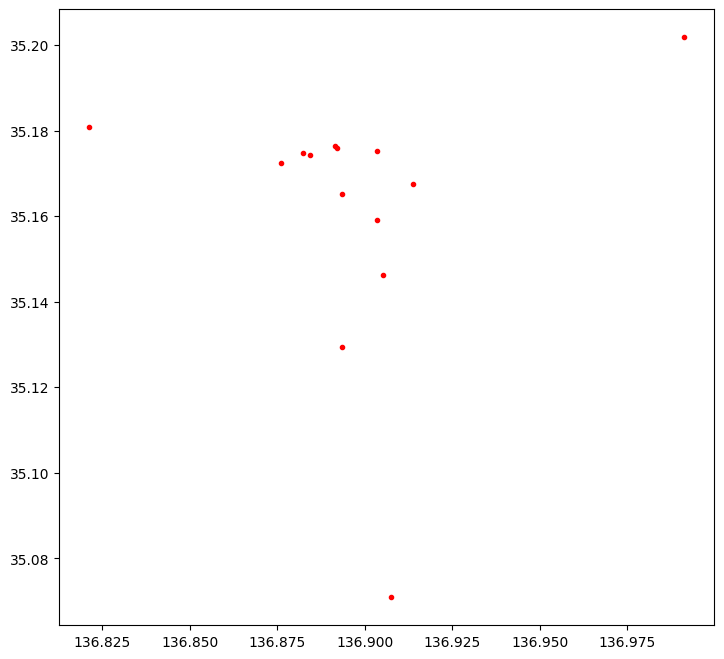
The red dots are the hostels in Nagoya.
Create a composite map using data from multiple shapefiles
Let’s mash up all the geospatial features covered so far and create a composite map of roads, riverbanks, and hostels in Nagoya city.
# Create a plot with specified size
fig, ax = plt.subplots(figsize=(10, 8))

# set the range of x-axis and y-axis
plt.xlim([bbox[0], bbox[2]])
plt.ylim([bbox[1], bbox[3]])

# Plot roads
roads[roads['fclass'].isin(["primary", "secondary", "tertiary", "service"])].plot(ax=ax,
                                                                                  linewidth=0.5,
                                                                                  color='black',
                                                                                  alpha=0.4)

# Plot riverbank
water[water['fclass'] == "riverbank"].plot(ax=ax, color = "steelblue")

# Plot hostels
pois[pois['fclass'] == "hostel"].plot(ax=ax, c = "red", marker='.')

My next objective is to create interactive maps using the same shapefile data in Python. Do let me know in the comments if you already know how to do that. Thanks for your time!