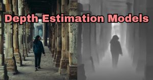
What is Depth Estimation?
Depth estimation is a fascinating field in computer vision that allows us to infer the distance of objects from a single image or a pair of images. Imagine being able to measure how far away things are just by looking at a photo!
At its core, depth estimation answers the question: “How far is that object?” It’s like having a magical ruler that can measure distances in a photograph. Whether you’re building self-driving cars, augmented reality apps, or even robots, understanding depth is crucial.
Monocular vs. Stereo Depth Estimation
There are two types of depth estimation approaches – Monocular depth estimation and Stereo depth estimation.
Monocular Depth Estimation
- Uses a single RGB image to estimate depth.
- Like having one eye closed and trying to judge distances.
- Commonly used in smartphones for portrait mode effects.
- Models: These models learn to predict depth directly from a single image.
Stereo Depth Estimation
- Uses two images (taken from slightly different angles) to estimate depth.
- Like having two eyes and using the parallax effect to gauge distances.
- Widely used in robotics and 3D reconstruction.
- Models: These models exploit the relationship between the two images to calculate depth.
In this article, we will focus on monocular depth estimation models only.
Depth estimation models in action
Let’s use a few state-of-the-art depth estimation models with the Hugging Face Transformers library and Python. I am using Google Colab and it has Transformers library pre-installed.
from transformers import pipeline
from PIL import Image
Load input images
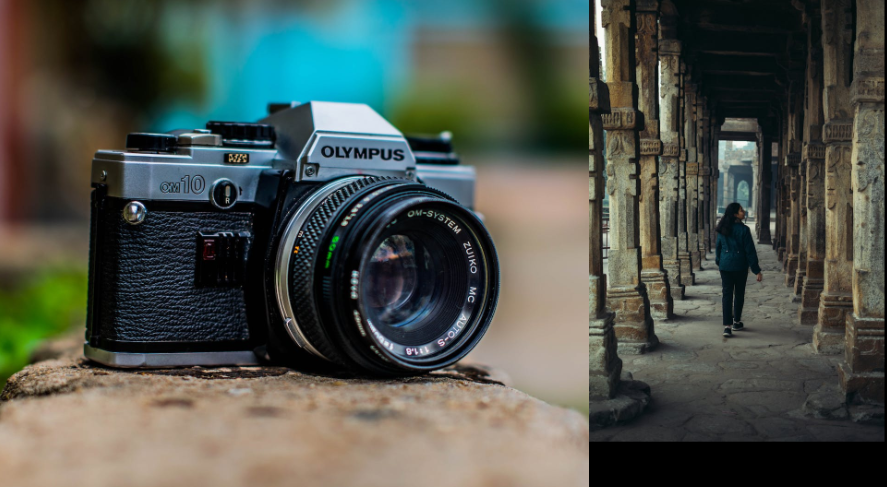
I will use two images for depth estimation. One image will have a close-up of an object and the other image is an architectural photograph.
# load input images
input_image1 = Image.open("img1.jpg")
input_image2 = Image.open("img2.jpg")

# function to display multiple images together
def image_grid(imgs, rows, cols):
    assert len(imgs) == rows * cols

    w, h = imgs[0].size
    grid = Image.new("RGB", size=(cols * w, rows * h))
    grid_w, grid_h = grid.size

    for i, img in enumerate(imgs):
        grid.paste(img, box=(i % cols * w, i // cols * h))
    return grid

#display images
image_grid([input_image1, input_image2], rows = 1, cols = 2)
Create a depth estimation pipeline
Before using a depth estimation model, I will create a function that will take an image and model name/path as inputs, use Transformers Pipeline to load the depth estimation model, and return depth-image as output.
def depth_estimator(img, model_path):
  # load depth estimation model
  pipe = pipeline('depth-estimation', model = model_path)

  # generate depth image
  depth_image = pipe(img)['depth']

  return depth_image
DPT-Large model
Let’s use the DPT-Large model for depth estimation for both the input images. This model was trained on 1.4 million images for monocular depth estimation.
depth_image1 = depth_estimator(input_image1, "Intel/dpt-large")

# display images
image_grid([input_image1, depth_image1], rows=1, cols=2)

depth_image2 = depth_estimator(input_image2, "Intel/dpt-large")

image_grid([input_image2, depth_image2], rows=1, cols=2)

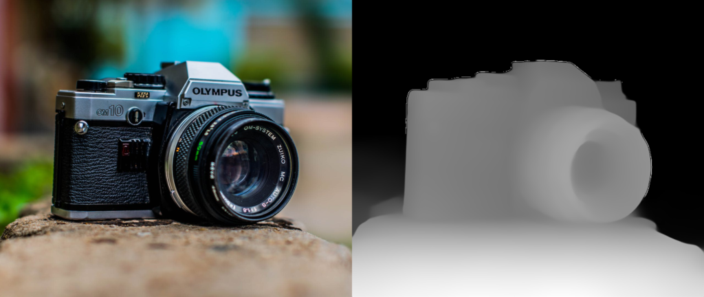
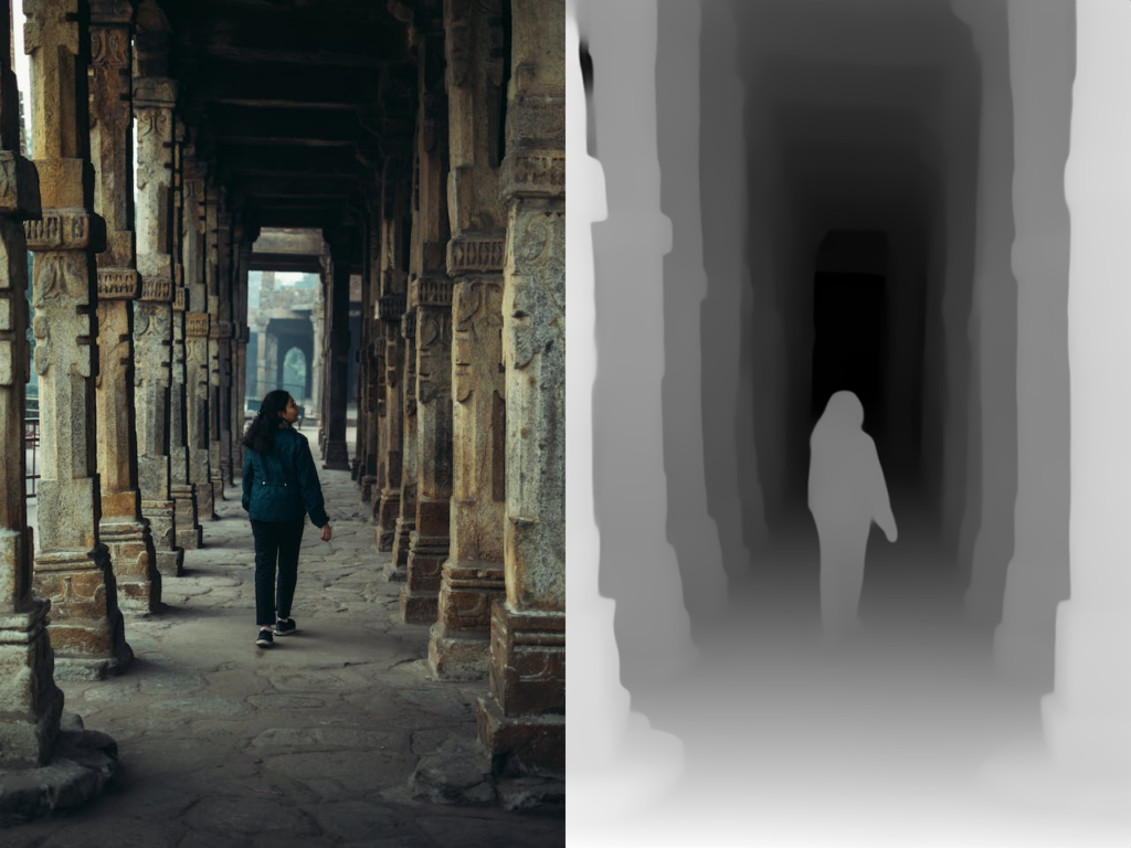
As you can see the depth images are grayscale images. The pixels of these images are darker for far-away objects and brighter for nearby objects.
The performance of a depth estimation model can be evaluated based on the level of detail captured by the model and how far it can estimate the depth in the input image.
DPT-Hybrid Midas
Let’s try another popular monocular depth estimation model.
depth_image1 = depth_estimator(input_image1, "Intel/dpt-hybrid-midas")

image_grid([input_image1, depth_image1], rows=1, cols=2)

depth_image2 = depth_estimator(input_image2, "Intel/dpt-hybrid-midas")

image_grid([input_image2, depth_image2], rows=1, cols=2)

The performance of the DPT-Hybrid Midas is slightly inferior to that of the DPT-Large model.
Depth Anything
Depth Anything family of models are lightweight models with similar or better performance than the models we have seen above. Let’s try out the base version of Depth Anything model.
depth_image1 = depth_estimator(input_image1, "LiheYoung/depth-anything-base-hf")

# display images
image_grid([input_image1, depth_image1], rows=1, cols=2)
depth_image2 = depth_estimator(input_image2, "LiheYoung/depth-anything-base-hf")

# display images
image_grid([input_image2, depth_image2], rows=1, cols=2)
GLPN fine-tuned on NYU
Global-Local Path Networks or GLPN uses the SegFormer framework and adds a lightweight head on top for depth estimation.
depth_image1 = depth_estimator(input_image1, "vinvino02/glpn-nyu")

image_grid([input_image1, depth_image1], rows=1, cols=2)

The depth-image for this model is inverted. That means the foreground pixels would be darker than the background pixels.
depth_image2 = depth_estimator(input_image2, "vinvino02/glpn-nyu")

image_grid([input_image2, depth_image2], rows=1, cols=2)
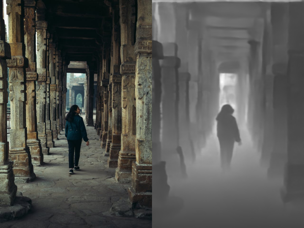
The performance of GLPN-NYU is not that great for the first image, but as you can see the depth estimation for the second image is quite good.
Conclusion
Depth estimation models open up a world of possibilities in computer vision. Whether you’re measuring the distance to a mountain peak or creating captivating augmented reality experiences, understanding depth is essential.
Remember, there’s no one-size-fits-all approach. Traditional methods rely on geometry, while learning-based models leverage neural networks.
